This code introduces how to perform parameter estimation for a system of differential equations in R. First, the necessary packages and data are imported using code previously introduced in a previous post. R code available here.
## load packages we need to run the functions
library("readxl")
library(deSolve)
library(nloptr)
library(reshape2)
library(minpack.lm)
# # # ## # # #
# Import Data
# # # ## # # #
## Paste this from your existing code
Due to computational constraints, the mathematical model we are using to fit to the data includes product inhibition. If product inhibition doesn’t exist in the data, then the inhibition parameter i will be estimated to be close to zero.
# # # ## # # #
# Parameters
# # # ## # # #
r = .001 #
i = 0.00001 #
f=10 #
S_mL=5 #
E_mL=1 #
ce = E_mL*f #
se = S_mL*f #
tmax = 180 #
The initial conditions, model equations, and plotting statements are then executed to visualize the initial parameter guesses.
# # # ## # # #
# Equations
# # # ## # # #
yini=c(S=se,P=0,E=ce) #
derivs = function(t,y,parms){
with(as.list(y),{
dS=-r*E*S #
dP=r*E*S-i*E*P#
dE=-i*E*P #
list(c(dS,dP,dE))
})
}

# # # ## # # #
# Calculate
# # # ## # # #
times = seq(from=0,to=tmax,by=15)
out = ode(y=yini,t=times,func=derivs,parms=c(r,i))
head(out) #

# # # ## # # #
# Plot initial guess
# # # ## # # #
plot(out[,"time"],out[,"P"]*1,type="l",lwd='3',col="bisque4",xlab="label (units)",ylab="label (units)",sub="Figure description",xlim=c(0,tmax),ylim=c(0,60))
lines(t,averages,type='p')
arrows(t, (averages+std_dev),t, (averages-std_dev), length=0.05, angle=90, code=3)
Next the fitting function ssq is defined. It takes a vector of the parameters p as an input. The value of the parameters will change with each iteration of the fit until the sum of squares stops changing very much. This will be a local optimum and give us our parameter estimates.
# # # ## # # #
# parameter fitting using levenberg marquart algorithm
# # # ## # # #
ssq=function(p){
# parameters from the parameter estimation routine
f=p[3]
r=p[1]
i=p[2]
print(p)
The parameters we will be estimating include the scaling parameter f, the reaction rate r, and the inhibition parameter i. The scaling parameter f alters the initial amounts of substrate and enzyme cinit. The amount of initial product can be manually changed to fit the data.
# inital concentration
cinit=c(S=as.numeric(5*f),P=0,E=as.numeric(1*f))
# time points for which conc is reported
# include the points where data is available
tvs=c(seq(0,180,30),my_data$TIME)
tvs=sort(unique(t))
Then the model is solved numerically using these parameters and initial conditions.
# solve ODE for a given set of parameters
out=ode(y=cinit,t=tvs,func=derivs,parms=list(r,i))
The time between data points can be long. Numerically solving the model only at these far apart time points can produce inaccurate results. So we solve the model over shorter time points and then take putt the simulation value at the same time points as our data in the vector outdf.
# Filter data that contains time points where data is available
outdf=data.frame(out)
outdf=outdf[outdf$time %in% my_data$TIME,]
times = c(outdf$time,outdf$time,outdf$time)
ys = c(outdf$P,outdf$P,outdf$P)

# Evaluate predicted vs experimental residual
preddf=data.frame(times,ys)
In our case, we only have data of the product, not the enzyme or substrate. So we concatenate the time points and the simulated product 3 times in the vectors times and ys. This is because our data exist in triplicate.
expdf=melt(c(my_data$'Rep 1__1',my_data$'Rep 2__1',my_data$'Rep 3__1')*(40/maxconc),id.var="time",variable.name="species",value.name="conc")#(my_data$Rep 1__1,my_data$Rep 2__1,my_data$Rep 3__1,*(40/maxconc),id.var="time",variable.name="species",value.name="conc")
ssqres=(preddf$ys-expdf$conc)
print(sum(ssqres)^2)

# return predicted vs experimental residual
return(ssqres)
}
In expdf we concatenate the data corresponding to our 3 replicates, multiplied by the same scaling factor used previously. The sum of squares function returns a vector of predicted minus actual differences. The R function nls.lm sums and squares it for us. We end the sum of squares function with a return statement and our differences vector.
# initial guess for parameters
p=c(.001,.0001,10)
# initial ssq
initial_res=ssq(p)
sum(initial_res)^2
Before calling the fitting function nls.lm, we provide our initial parameter guesses in the vector p, and get the initial sum of squared residuals initial_res. This is so we can quantify how much the fit improved when we used a fitting algorithm, compared to the fit we obtained by hand.
# fit model - return sum of squares and parameters at each iteration
fitval=nls.lm(par=p,lower=c(0.00001,0.000001,1),upper=c(0.1,.01,20),fn=ssq)
# improvement in fit:
(sum(initial_res)^2 - 41.4)/sum(initial_res)^2
Finally, we call the fittting function nls.lm. We pass our parameter vector p along with lower and upper boundaries on the parameters. We know that biological parameters can’t be less than zero, and its doubtful that the scaling factor would be less than 1. However, if parameter estimates come close to the boundary, that is a good reason to alter the boundary values to be more conservative.
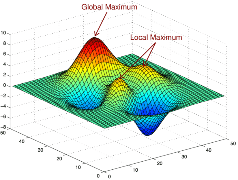
Keep in mind that this method produces local estimates of the parameter values. Local estimates mean that it is sensitive to initial guesses and boundaries placed on the parameters. A global estimate would produce the ‘absolute’ best estimates for the parameters, by virtue of creating a very small difference between the model and the data. In this case, we wouldn’t benefit very much by obtaining a global estimate, so a local estimate will do fine. IT is better to understand the importance of these numbers rather than getting the objectively best parameter estimate for learning purposes.
# # # ## # # #
# Plot fitted model
# # # ## # # #
r = fitval$par[1]
i = fitval$par[2]
f = fitval$par[3]
cinit=c(S=as.numeric(5*f),P=0,E=as.numeric(1*f))
legend("topleft",legend=c("Initial Guess","Fitted Model"),col=c("bisque4","bisque2"),pch=c(1,1))
out=ode(y=cinit,times=t,func=derivs,parms=c(r,i))
lines(out[,"time"],out[,"P"]*1,type="l",lwd='3',col="bisque2")
outdf=data.frame(out)
names(outdf)=c("time","ca_pred","cb_pred","cc_pred")
Finally, the simulation using the new fitted parameters is plotted against the data and model with the initial guess to visualize the improvement when using the fitting function.
