Introduction to an Introduction to Approximate Bayesian Computation (ABC)

Last week I re-blogged a post introducing Approximate Bayesian Computation. I thought some of the content was a little foreign, so I wanted to give an intro to the intro.

ABC core concept

Say we have a process that is controlled by a parameter – say the slope in , or the probability of observing a success. Under frequentist statistics (the regular kind), we assume that that parameter has a singular value, and we estimate it based on the data we observe. Under Bayesian statistics, the parameter comes from a distribution of possible values.

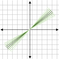
This is generally more realistic, since variability affects all aspects of life – machine error, incorrect assignment, temperature fluctuations, etc. All these factors introduce variability into a system, and a model of that system would be more accurate if it could include variable ‘rules’ (ie, parameters).

If that’s the case, why doesn’t everyone use Bayesian statistics? Well, its computationally very difficult, and only really feasible with recent technology, particularly for complicated models that aren’t even statistical distributions.

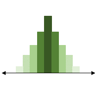
Traditional Bayesian statistics takes a prior distribution of the parameter (what we know or think a parameter’s values will likely be) and the likelihood distribution of the data given the parameter (for some parameter values, the data are more likely observed). Usually the likelihood is a statistical distribution – like the probability of a coin flip being heads. But what if we want to estimate the slope ? That isn’t a good likelihood, it isn’t a distribution. That’s where Approximate Bayesian Computation comes in.

Approximate Bayesian Computation (ABC)

We can approximate a likelihood distribution using our model of the slope . All we need to do is figure out how to calculate the likelihood. For a real likelihood distribution, we calculate how likely / probable the data are given a parameter’s value.

To approximate this, we can calculate how different is from for and . This allows us to calculate how the different parameter values for m affect the data. This isn’t exactly the same value, but it’s analogous, and more importantly it works!

Of course, this relies on a good choice for how we calculate the difference between y_model and y_data. In real applications, we will have multiple parameters and even multiple y’s and x’s that can all take different values. We may know how accurate our measures are of y and x, and this may even be happening over time. So our choice of how we calculate the difference is difficult and important.

Sampling routine

With this information, let’s look at the rejection sampling algorithm mentioned in the blog post:

1. Pull a random value of the model parameter(s) from the prior distribution on the parameter(s)
2. Obtain model evaluation using the parameters from step 1
3. Compute the difference between simulation and data; reject if difference is too large
4. Repeat

In the introduction blog, the Euclidean distance is used (sum squared difference between model and data); although other distance formulations may be more appropriate – [2] uses the ‘energy statistic’, which calculates the distance in multi-dimensional space. (Euclidean distance is better for lower dimensional spaces; so if you have many parameters to estimate, a different distance metric would work better.)

Example application

The blog post gives an example using the Lotka-Volterra equations. This is a standard model often used to illustrate methods, since it’s mathematically simple with complex dynamics.

The Lotka-Volterra model represents the back-and-forth between predator and prey in an ecological setting. The model has two variables (predator, prey) and four parameters (predator growth thanks to prey, and death; prey birth, and death due to predation). The dynamics oscillate as predators increase; run out of resources and drop; while prey increase, until resources are plentiful; etc. The model will always oscillate, although the shape of those oscillations depends on model parameters.

In this case, you may be able to imagine that a given species of predator and its prey might have generally true properties that parameters can describe. However, this is over generational time – seasons, competition, and other random effects might alter what that parameter value is specifically. For example, if a prey is white and there is more snow than usual, then the parameter controlling successful prey capture might be lower for part of the simulation.

Estimating the distribution that the parameter comes from is useful and realistic; and we could use the variability of that distribution to compare this system to other predator-prey systems, obtaining additional biological inference.

Simulation-based inference

The blog post provides some code for running the ABC algorithm with the Lotka-Volterra model by coding it yourself. This is one method to implementing ABC – some “pre-packaged” implementations will try to improve performance by approximating the likelihood as quickly as possible. Since we use the prior to randomly generate new parameter values, calculating the difference between model and data is the limiting step of ABC inference. Other methods to approximate the likelihood include using likelihood ratios (limits calculations, [2]); there are many other methods, including various datamining techniques such as neural networks [3]. I currently know of two packages for Python that use the likelihood-ratio method (sbi and delfi) – let me know if you are aware of other packages!

References:

1. Nguyen H.D. (2019) An Introduction to Approximate Bayesian Computation. In: Nguyen H. (eds) Statistics and Data Science. RSSDS 2019. Communications in Computer and Information Science, vol 1150. Springer, Singapore. https://doi.org/10.1007/978-981-15-1960-4_7
2. Hermans, J., Begy, V. & Louppe, G. Likelihood-free MCMC with Amortized Approximate Ratio Estimators. arXiv:1903.04057 [cs, stat] (2020).
3. Cranmer, K., Brehmer, J. & Louppe, G. The frontier of simulation-based inference. Proc Natl Acad Sci USA117, 30055–30062 (2020).

More info:

1. Heinemann, T. & Raue, A. Model calibration and uncertainty analysis in signaling networks. Current Opinion in Biotechnology39, 143–149 (2016).