
It’s been quite a while since I updated this tutorial series- better late than never?
Introduction
First, we determine the distribution our data comes from, or the likelihood, and any prior information is described using the prior distribution. Then we use Markov chain Monte Carlo to explore this posterior. Then we determine if we need Metropolis-Hastings or Gibbs sampler, or both. Now we are ready to code in R!
Sampling in R
First you’ll need to load the Marko chain Monte Carlo package:
library(MCMCpack)
Then import data, or draw randomly.
# # example random dataset
d1=rgamma(10,1,.2)
d2=rgamma(10,1,.5)
d3=rgamma(10,1,.7)
data=c(d1,d2,d3)
We can visualize & summarize our data using
hist(data)
mu=mean(data);v=mean(var(data))
Now we specify priors. For this example, I want to use a Gamma distribution on t and k, with initial estimates of 1.
t0=1;k0=1
alpha0=.1;beta0=.1

tprior=function(alpha0,beta0,t){
 dgamma(t,shape=alpha0,scale=beta0)
}
kprior=function(alpha0,beta0,k){
 dgamma(k,shape=alpha0,scale=beta0)
}
Then we code the likelihood.
likelihood=function(ti,1,x,n){
 like=1
 for (i in 1:n){
  like=like*dgamma(x[i],shape=1,scale=ti) # numerical way to obtain  likelihood
 }
 like # the value is returned by the function
}
Then we code the posterior, which is the priors multiplied by the likelihood.
posterior=function(beta0,alpha0,ti,ki,x,n){
 tprior(beta0,alpha0,ti)*kprior(beta0,alpha0,ki)*likelihood(ti,ki,x,n)
}
Finally, Markov chain Monte Carlo. This uses a random walk from the current parameter value to a random value within the proposal distribution. The number of times a parameter sits at a given value corresponds to higher probability density at that value, since the posterior probability will be higher as the parameter approaches the true value supported by the likelihood and the data.
The figure above illustrates the concept of the random walk along the posterior (from here). Here I’m using Gibbs within Metropolis Hastings for illustration. Comments with additional details are provided in green.
sample=10000

gibb.sample=matrix(0,sample,2) # save values from each iteration

tmu=c(t0,k0) # current parameter estimates = alpha, lambda

var_star = 0 # dummy variable for each iter

n=as.numeric(nrow(data)) # size of dataset

sd.rw=c(.01,1) # controls variance of proposal distribution (lambda is prob <1)

accept=matrix(0,1,2) # acceptance matrix ~ 20%

# # # # # # #

#each iteration, update the matrix of starting values

for(j in 1:sample){

# # # # a #

var_star <- rtnorm(1,tmu[1],sd.rw[1],0) #proposal distribution - truncated normal

nom=posterior(beta0,alpha0,var_star,tmu[2],data,n)

denom=posterior(beta0,alpha0,tmu[1],tmu[2],data,n)

alpha <- min(1, nom/denom) # compare probability density at new and old parameter value


r <- runif(1,0,1) # we accept possible parameter values if alpha is larger than a random number from a uniform

if (r<=alpha ) {

 accept[1] <- accept[1]+1

 tmu[1] <- var_star # next iteration we'll draw from the proposal distribution centered at the current value

}

gibb.sample[j,1]=var_star


var_star <- rtnorm(1,tmu[2],sd.rw[2],0)

nom=posterior(beta0,alpha0,tmu[1],var_star,data,n)

denom=posterior(beta0,alpha0,tmu[1],tmu[2],data,n)

alpha <- min(1, nom/denom)

r <- runif(1,0,1)

if (r<=alpha ) {

accept[2] <- accept[2]+1

tmu[2] <- var_star

}

gibb.sample[j,2]=var_star

}

accept[]/sample # check for reasonable - 20-60% ish
The acceptance rate tracks how often we move from the current parameter value to the proposed value. We don’t want to get stuck at a local minimum, and sometimes the posterior distribution can be complex, including multimodal distributions.
An acceptance rate that is too high means that the samples will not converge to the posterior. In this case, the proposal distribution is likely too thin, so that every value the proposal distribution draws is within the posterior. On the other hand, an acceptance rate that is too low may mean that the proposal distribution is too wide, meaning there is a higher probability that we will draw a proposed value for a parameter that is outside the posterior distribution. The suggested acceptance rate is 20%, but this is specific to the complexity of the problem among other concerns.
Finally, plot the samples over all iterations for each of the parameters. These plots are called trace plots. Check for convergence and find the appropriate throwaway rate.
plot(gibb.sample[,1]) # look for convergence and find the throwaway rate
plot(gibb.sample[,2])
trash=1000
mean(gibb.sample[trash:sample,1])
var(gibb.sample[trash:sample,1])
mean(gibb.sample[trash:sample,2])
var(gibb.sample[trash:sample,2])
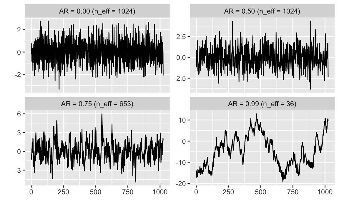
The figure below (from here) gives you some idea of what convergence looks like in the trace plots. The top two examples show clear convergence. Imagine drawing a distribution curve along the y axis – some ‘outliers’ are part of the tails of the distribution! The bottom left is possibly converged, and the bottom rate shows an acceptance rate that is too high.
Next I’ll talk about Bayesian hypothesis testing, and a tool I’ve been working on to make it more accessible to non-Bayesians!
