Computational Plant Science – Clustering in R Tutorial

Last week was the Plantae Seminar “Computational Plant Science – Science at the Interface of Math, Computer Science, and Plant Biology with Alexander Bucksch”:

Dr. Bucksch mentions using two clustering techniques – B splines and K-means clustering. I’ve discussed K-means clustering in a previous post to analyze predictors of success in Settlers of Catan.

B splines

Background

B splines are used to fit curves. Their predictive power is restricted to the range of the data that is fitted.

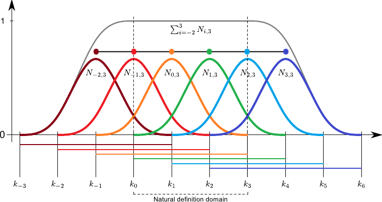
B splines are defined over a basis, or number of discrete points along an axis. Basis functions are defined over 3 points, overlapping. Basis functions can be linear, producing ‘triangles’, or some degree of polynomial, such as second-degree in the image above. The fit is the sum of the basis functions at each point along the axis.

R code

Try out the following code in R. You can download R here​. You can get the relevant spline packages here, or more examples and example code here.

The kyphosis data is non-numeric, so first we must convert to binary. Since the data are binary, we use the binomial distribution to fit.

load('kyphosis.Rdata') source('bases.r') source('ps_binomial.r')
x = kyphosis$Age y = 1 * (kyphosis$Kyphosis == 'present') # make y 0/1

The tuning parameter, lambda, determines how ‘fitted’ the result is to the data. Overfitted models are poor at prediction, and underfitted models are poor at capturing trends in the data. You can see my previous discussion on model fit here.

# optimise lambda 
lla = seq(-2, 10, by = 0.2) 
aics = 0 * lla 
for (k in 1:length(lla)) { 
lambda = 10 ^ lla[k]
 pp = ps.binomial(x, y, nseg = 20, lambda = lambda, plot = F) 
aics[k] = pp$aic 
} 
plot(lla, aics, xlab = 'log10(lambda)', ylab = 'CV') 
lines(lla, aics) lambda=1^1.8 
#optimal lambda is 1^1.8

Now we can perform a B spline fit. We have chunked the x-axis into 20 segments, chosen a basis function of order 3, and determined our best fitting parameter.

pf=ps.binomial(x,y,nseg=20,bdeg=3,pord=2,lambda=1^1.8)

K-means

Background

K-means clustering is unsupervised, meaning the algorithm identifies relationships within a data set without a response variable. This makes it useful to use in conjunction with other analyses, such as B splines. For Dr. Bucksch’s analysis, he likely clustered B spline fitting parameters to determine which conditions resulted in similar fits.

The algorithm works by calculating the distance of all data points from the center of each cluster, which is re-defined during each iteration. The number of clusters can be determined by cross-validation, or reducing the mean squared error, or a priori.

R code

First load in the data. I am using the Settlers of Catan dataset from Kaggle.

data=read.csv('catanstats.csv')

Then set the seed and set the maximum number of clusters. Since there are 25 variables in the dataset, I set this to 25.

set.seed(124)
k.max=25

Then determine the ideal number of clusters using cross validation by performing K-means on 1 : 25 clusters. Plot the number of clusters by the total sum of squares and look for the point at which there is a significant reduction in the sum of squares. Unlike other methods, you aren’t looking for the minimum – the sum of squares will almost always be reduced as you increase the number of clusters, but this is overfitting and results in poor prediction.

data=quantdat[,-1]
wss=sapply(1:k.max,function(k){kmeans(data,k,nstart=50,iter.max=15)$tot.withi
nss})

plot(1:k.max,wss, type="b", pch = 19, frame = FALSE, xlab="Number of clusters K", ylab="Total within-clusters sum of squares")

Now you can perform K-means clustering on the data, where 2 is the number of clusters, and 50 is the total number of 2-way clusters I need to observe all 25 variables.

clusters=kmeans(data[,-1],2,nstart=50)
plot(data[,-1], col =(clusters$cluster +1) , main="K-Means result with 2
clusters", pch=20, cex=2)