As mentioned in Part 1, in Bayesian statistics you summarize a priori knowledge in the prior, and your data in the likelihood. The prior distribution is often chosen based on analytical convenience, while the likelihood is chosen based on the underlying sampling distribution (read about some appropriate distributions here). Multiplying these together produces the posterior distribution.

Probability distributions are nice equations that allow us to obtain their true means and variances. Frequently, depending on the prior and the likelihood, as well as the problem itself, the posterior distribution can’t be derived directly. In this case we can use Markov chain Monte carlo to describe it numerically.
Markov chain Monte Carlo (MCMC)
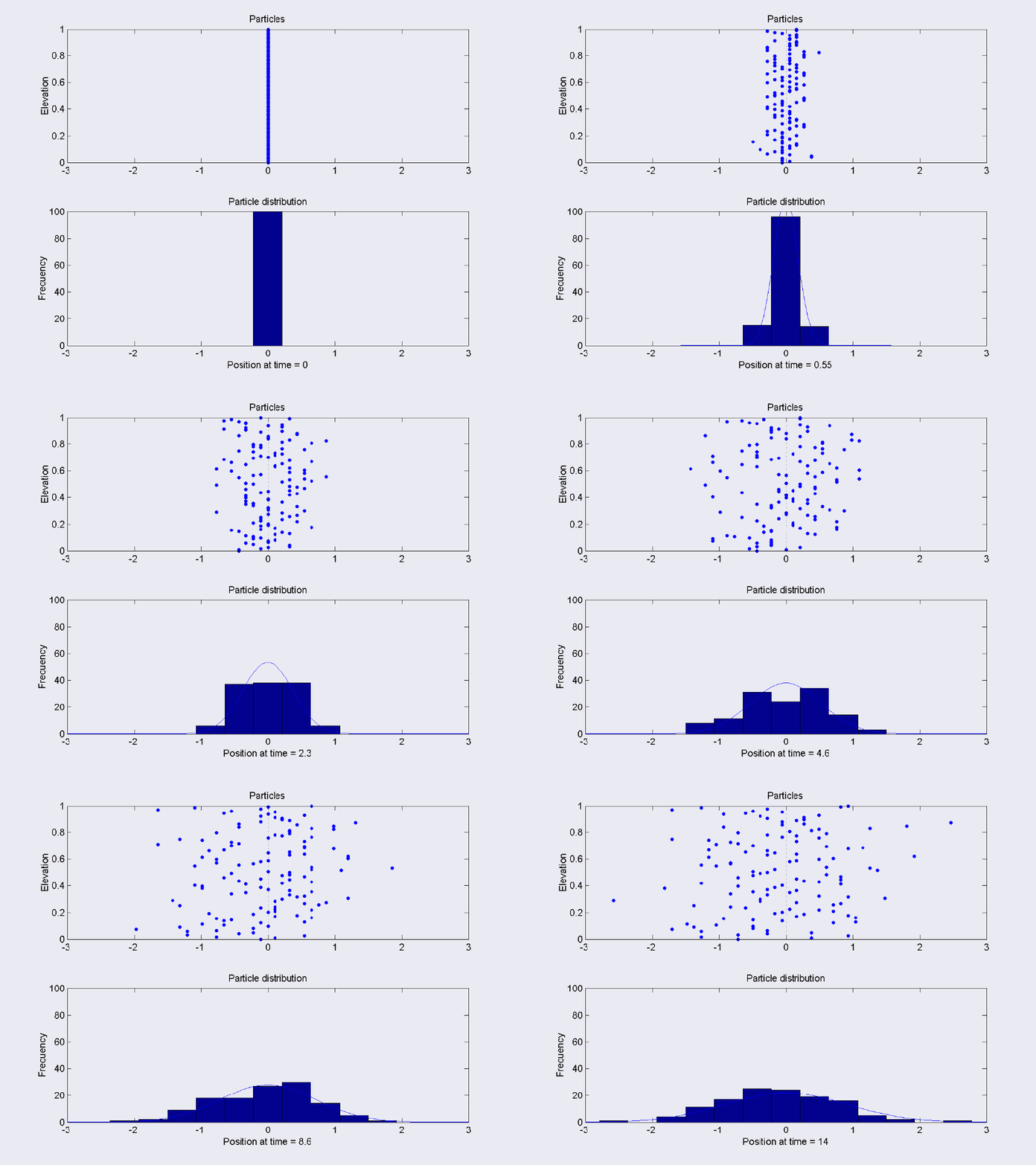
MCMC iteratively samples from your posterior function using a random walk.

The posterior function is some kind of distribution. To understand how a random walk helps construct the posterior, imagine a symmetric distribution such as a Normal. The middle of the Normal is equivalent to the median, or most likely value. As you move towards the edges of the distribution, the chance of observing the values decreases.
Random walks can be used to flesh out the posterior distribution numerically. Beginning at a random point on the line,
- Randomly draw a value from the proposal distribution.
- Compute the posterior (prior * likelihood) at the current random point, and the new proposed point.
- If the new, proposed point has a higher probability than the current point, randomly draw a value from a uniform distribution.
- If the probability of the new point is >= the random uniform value, the proposed point becomes your new position.
- Repeat.
The proposal distribution is usually a Normal distribution, although it can be a Beta or a Uniform. Considering the Normal case, since the distribution is centered at your current point, a value very close to the current point is highly likely to be drawn at random. The variance of the Normal distribution is known as the tuning parameter. The tuning parameter allows you to make it more or less likely to choose a point close to your current position.
The uniform distribution is a flat distribution. In this case, it is between 0 and 1. Every point is equally likely – so this value has equal chance to be 0.01 as 0.99.
By manipulating the tuning parameter, you can obtain a faster or slower exploration of the posterior distribution. Eventually, you will move from your current point, with some probability x of being observed within your posterior, to the median of the posterior. The median has the highest probability of being observed, so it is less likely that the value drawn at random from the uniform distribution will be greater. This means that you will be selecting this point very frequently – this leads to a numerical description of your posterior.
In part 3 we will discuss different algorithms for MCMC simulation: the Gibbs sampler and Metropolis Hastings.
