Curve fitting to multiple equations simultaneously

The simplest way to curve fit multiple equations while conserving some parameter values is by converting the problem into matrix form. For example, for a set of two equations such as:

$\frac{ d X(t)}{ d t}= - \alpha X(t) -\gamma Z(t)\\ \frac{ d Y(t)}{d t}=\alpha W(t)-\epsilon Y(t)$

we may write the solution matrix as:

$\begin{Bmatrix} -\alpha & -\gamma \\ \alpha & -\epsilon \end{Bmatrix}$

Curve fitting functions are generally using local optimization techniques such as minimizing sum of squares.

$\sum_{i=1}^n (X(i)-x_i)^{2}$

Here, i is the solution of the X equation at the $i^{th}$ time point and the corresponding data point.

We can exploit this to miminize a matrix of values by providing a matrix of data and a matrix of solutions. For data sets corresponding to X and Y, concatenate the vectors into a matrix:

$\begin{Bmatrix} X & \cdots & \cdots \\ Y & \cdots & \cdots \end{Bmatrix}$

The output of the solutions to X(t) and Y(t) with the current set of parameter values can also be put into a matrix. Then the sum of squares can be solved on the matrices, allowing for parameter values to be conserved across equations.

$\sum_{i=1}^n (\mathbf M(i)-\mathbf V_i)^{2}$

where M and V are the parameter and data matrices respectively.

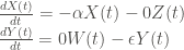
For the initial estimates of the parameters, I’ve had success with separately curve fitting each equation separately in a user-friendly software such as JMP. For difficult equations such as logarithms, I’ve found that setting a selection of parameters to zero allows for good initial estimates. In this example system:

$\frac{ d X(t)}{ d t}= - \alpha X(t) - 0 Z(t)\\ \frac{ d Y(t)}{d t}=0 W(t)-\epsilon Y(t)$

Share this:

Like this:

Related

Leave a Reply Cancel reply